44 align data labels in excel chart
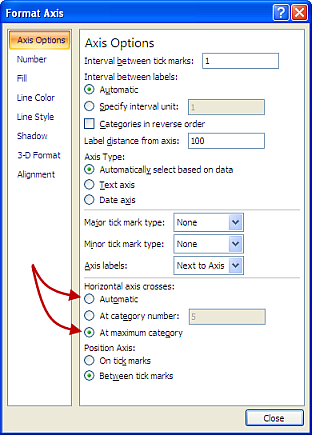
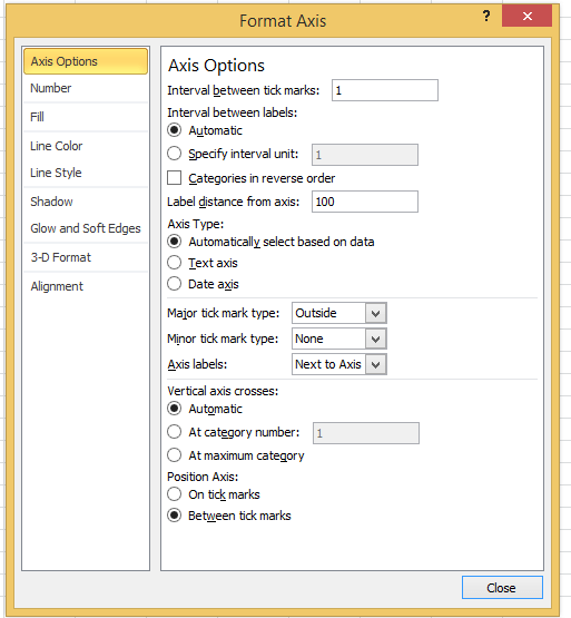
How to Create and Customize a Funnel Chart in Microsoft Excel Open your spreadsheet in Excel and select the block of cells containing the data for the chart. Head to the Insert tab and Charts section of the ribbon. Click the arrow next to the button labeled Insert Waterfall, Funnel, Stock, Surface, or Radar Chart and choose "Funnel.". The funnel chart pops right into your spreadsheet. Date Axis in Excel Chart is wrong • AuditExcel.co.za In order to do this you just need to force the horizontal axis to treat the values as text by. right clicking on the horizontal axis, choose Format Axis. Change Axis Type to be Text. Note that you immediately lose the scaling options and the date scale puts in exactly what is in the data, onto the horizontal axis.
› article › technology5 New Charts to Visually Display Data in Excel 2019 - dummies Aug 26, 2021 · Select the data and labels and then click Insert → Maps → Filled Map. Wait a few seconds for the map to load. Resize and format as desired. For example, you could apply one of the chart styles from the Chart Tools Design tab. To add data labels to the chart, choose Chart Tools Design → Add Chart Element → Data Labels → Show. Pouring ...

Align data labels in excel chart
Excel Charts with Shapes for Infographics - My Online Training Hub How to Build Excel Charts with Shapes Start by inserting a regular column chart. Then insert the shape you want to use. Make sure it's roughly the same size as the largest column in your chart. CTRL+C to copy the Shape > Select the columns in the chart > CTRL+V to paste the shape. Tip: add data labels and remove the gridlines and vertical axis. Tree Maps Data Labels and Tables Formatting/Sorting Errors after ... Tree Maps Data Labels and Tables Formatting/Sorting Errors after Windows 11. My Tree Map in Excel and Powerpoint after the Windows 11 update does not order my tables from smallest/largest value correctly, nor allow me to right-align my data labels, nor does it spell out the data label name. How to Overlay Charts in Microsoft Excel - How-To Geek In the Change Chart Type window, select Combo on the left and Custom Combination on the right. Create your chart: If you don't have a chart set up yet, select your data and go to the Insert tab. In the Charts section of the ribbon, click the drop-down arrow for Insert Combo Chart and select "Create Custom Combo Chart."
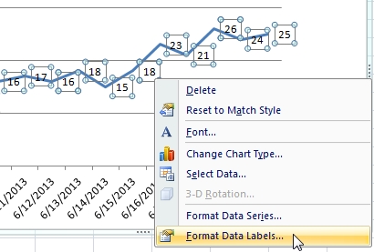
Align data labels in excel chart. Excel Chart VBA - 33 Examples For Mastering Charts in ... - Analysistabs We can create the chart using different methods in Excel VBA, following are the various Excel Chart VBA Examples and Tutorials to show you creating charts in Excel using VBA. 1. Adding New Chart for Selected Data using Sapes.AddChart Method in Excel VBA. The following Excel Chart VBA Examples works similarly when we select some data and click ... Make Excel charts primary and secondary axis the same scale First create 2 new columns and call then Primary and Secondary Scale. In the first cell create a MIN function that looks at ALL the original data points and finds the smallest number. In the last cell do the same but this time a MAX to find the biggest number out of all the data points. In E8 and E34 just equals to the adjacent cells. › excel › how-to-add-total-dataHow to Add Total Data Labels to the Excel Stacked Bar Chart Apr 03, 2013 · Step 4: Right click your new line chart and select “Add Data Labels” Step 5: Right click your new data labels and format them so that their label position is “Above”; also make the labels bold and increase the font size. Step 6: Right click the line, select “Format Data Series”; in the Line Color menu, select “No line” Chart.Axes method (Excel) | Microsoft Learn Syntax expression. Axes ( Type, AxisGroup) expression A variable that represents a Chart object. Parameters Return value Object Example This example adds an axis label to the category axis on Chart1. VB With Charts ("Chart1").Axes (xlCategory) .HasTitle = True .AxisTitle.Text = "July Sales" End With
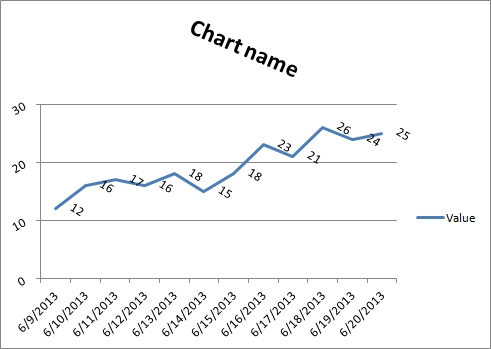
Custom Chart Data Labels In Excel With Formulas Select the chart label you want to change. In the formula-bar hit = (equals), select the cell reference containing your chart label's data. In this case, the first label is in cell E2. Finally, repeat for all your chart laebls. If you are looking for a way to add custom data labels on your Excel chart, then this blog post is perfect for you. › how-to-make-charts-in-excelHow to Make Charts and Graphs in Excel | Smartsheet Jan 22, 2018 · To generate a chart or graph in Excel, you must first provide the program with the data you want to display. Follow the steps below to learn how to chart data in Excel 2016. Step 1: Enter Data into a Worksheet. Open Excel and select New Workbook. Enter the data you want to use to create a graph or chart. How to change the orientation of all chart column labels simultaneously ... Add the labels and set the rotation as you desire. Select the entire chart you just created. Ctrl-C. Select the chart that contains all the series and remove all data labels. On the Home ribbon, press Paste, Paste Special..., Formats. The chart should now have labels in the same orientation for all series. Label line chart series - Get Digital Help Double press with left mouse button on the cell that contains the data label. Put the prompt between the words. Press Alt + Enter. Press Enter. Back to top 3. Align data labels If you want the labels to be aligned to the left simply select the data label. Go to tab "Home" on the ribbon. Press with left mouse button on the "Align Left" button.
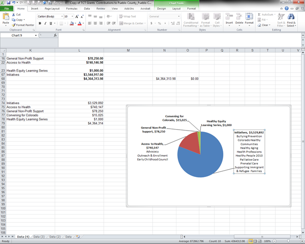
Align Chart Title in Excel - Explained! - Analysistabs The following step by step approach will help you to align the chart title position in the Excel Charts. Align Chart Title in Excel - Step 1: Select a Chart title You can activate any chart and select the chart title to re position the title. The below screen shot will show you how to select the chart title. Format and align chart title How to Change Chart Data Range in Excel (5 Quick Methods) - ExcelDemy Now, you want to change the chart data range. Firstly, you must Right-Click on the chart. Secondly, from the Context Menu Bar >> you need to choose Select Data. After that, you will see the following dialog box of Select Data Source. Now, from the dialog box of Select Data Source, you have to choose the Edit feature under the Sales option. Adding Data Labels to Your Chart (Microsoft Excel) - ExcelTips (ribbon) Activate the chart by clicking on it, if necessary. Make sure the Design tab of the ribbon is displayed. (This will appear when the chart is selected.) Click the Add Chart Element drop-down list. Select the Data Labels tool. Excel displays a number of options that control where your data labels are positioned. Select the position that best fits ... › how-to-create-excel-pie-chartsHow to Make a Pie Chart in Excel & Add Rich Data Labels to ... Sep 08, 2022 · In this article, we are going to see a detailed description of how to make a pie chart in excel. One can easily create a pie chart and add rich data labels, to one’s pie chart in Excel. So, let’s see how to effectively use a pie chart and add rich data labels to your chart, in order to present data, using a simple tennis related example.
How to move chart X axis below negative values/zero/bottom in ...
How to show all detailed data labels of pie chart - Power BI 1.I have entered some sample data to test for your problem like the picture below and create a Donut chart visual and add the related columns and switch on the "Detail labels" function. 2.Format the Label position from "Outside" to "Inside" and switch on the "Overflow Text" function, now you can see all the data label. Regards ...
How to align or rotate chart titles in Excel | Excel-example.com
peltiertech.com › excel-column-Column Chart with Primary and Secondary Axes - Peltier Tech Oct 28, 2013 · The second chart shows the plotted data for the X axis (column B) and data for the the two secondary series (blank and secondary, in columns E & F). I’ve added data labels above the bars with the series names, so you can see where the zero-height Blank bars are. The blanks in the first chart align with the bars in the second, and vice versa.
How to align or rotate chart titles in Excel | Excel-example.com
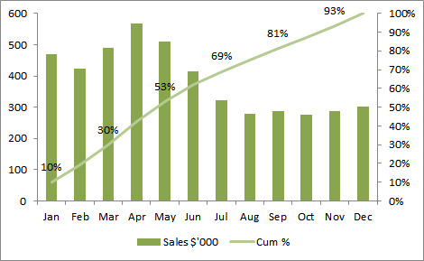
Excel Waterfall Chart: How to Create One That Doesn't Suck - Zebra BI Ideally, you would create a waterfall chart the same way as any other Excel chart: (1) click inside the data table, (2) click in the ribbon on the chart you want to insert. ... in Excel 2016 Microsoft decided to listen to user feedback and introduced 6 highly requested charts in Excel 2016, including a built-in Excel waterfall chart.
Align data labels in a graph so they are all along the same ...
Two-Level Axis Labels (Microsoft Excel) - ExcelTips (ribbon) Place your row labels into column A, beginning at cell A3. Place your data into the table, beginning at cell B3. With your table completed, you are ready to create the chart. Just select your data table, including all the headings in the first two rows, then create your table.
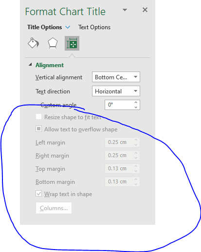
Excel: Formatting Chart Title: Alignment section is greyed ...
Formatting Long Labels in Excel - PolicyViz Simply place your cursor in the formula bar where you want to add the break and press the ALT+ENTER keys. Hit ENTER again, and you'll see the text wrap on two lines. You now have the text arranged the way you like it in the spreadsheet and in the graph. Aligning Labels
Quickest Way to Select and Align Charts for an Excel Dashboard
How to Make a Comparison Chart in Excel (4 Effective Ways) - ExcelDemy Let's learn the detailed steps to create a Comparison Chart using Scatter Chart. Steps: First, select the entire dataset. After that, go to the Insert tab. Then select Insert Scatter (X, Y) or Bubble Chart. Afterward, choose Scatter from the drop-down.

Chart Elements in Excel VBA (Part 2) - Chart Series, Data ...
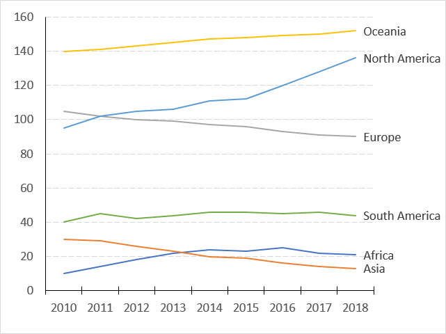
how to improve a line chart in Excel — storytelling with data Expand the 'Tick Marks' menu and select 'Outside' from the 'Minor type' drop-down menu. Let's also add tick marks to the x-axis and align the tick marks with the data points on the line by choosing 'On tick marks' under the 'Axis position' option.
Text Labels on a Horizontal Bar Chart in Excel - Peltier Tech
› how-create-waterfall-chart-excelHow to Create a Waterfall Chart in Excel and PowerPoint Mar 04, 2016 · To format the labels, select one of the labels, right-click, and select Format Data Labels from the list. Once the Format Data Labels pane opens, you can adjust the label position, text color and font to make the numbers more readable. *Once you’re done labeling the columns, you can delete unnecessary elements like zero values and the legend.
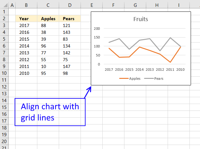
How to align chart with cell grid
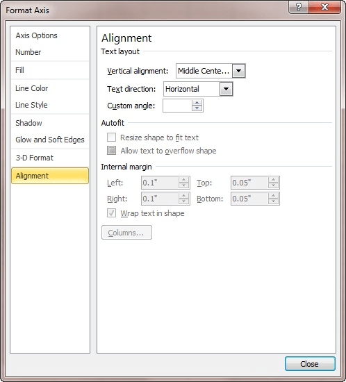
Can you change the text alignment of a Data Table in a Pivot Chart? You want the labels "Junk Data #" to be rotated 90 degrees. Right click on one of the data labels, to select the whole block Select "Format Axis" option to display the Format Axis Pane In the Format Axis pane > Axis Options > Size & Properties (3rd hieroglyphic icon) > Text Direction > pick which way you want to rotate it. Report abuse
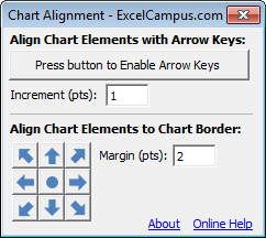
Move and Align Chart Titles, Labels, Legends with the Arrow ...
Data Labels in Excel Pivot Chart (Detailed Analysis) Add a Pivot Chart from the PivotTable Analyze tab. Then press on the Plus right next to the Chart. Next open Format Data Labels by pressing the More options in the Data Labels. Then on the side panel, click on the Value From Cells. Next, in the dialog box, Select D5:D11, and click OK.
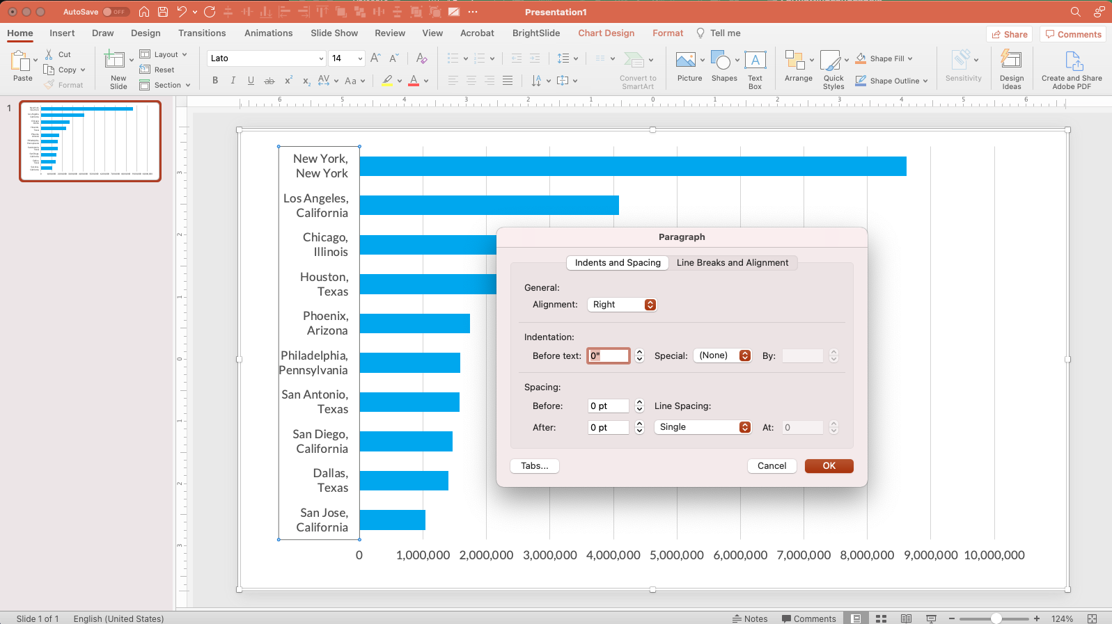
Formatting Long Labels in Excel - PolicyViz
Controlling Chart Gridlines (Microsoft Excel) - ExcelTips (ribbon) In the Current Selection group, use the drop-down list to choose the gridlines you want to control. Click the Format Selection tool, also within the Current Selection group. Excel displays a Format task pane at the right side of the program window. Use the controls in the task pane to make changes to the gridlines, as desired. Close the task pane.

How to Modify Cell Alignment & Indentation in Excel Video
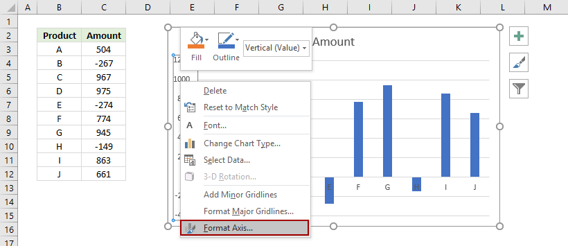
Format Chart Axis in Excel - Axis Options Analyzing Format Axis Pane. Right-click on the Vertical Axis of this chart and select the "Format Axis" option from the shortcut menu. This will open up the format axis pane at the right of your excel interface. Thereafter, Axis options and Text options are the two sub panes of the format axis pane.

Axis Labels overlapping Excel charts and graphs • AuditExcel ...
How to Print Labels from Excel - Lifewire To label legends in Excel, select a blank area of the chart. In the upper-right, select the Plus ( +) > check the Legend checkbox. Then, select the cell containing the legend and enter a new name. How do I label a series in Excel? To label a series in Excel, right-click the chart with data series > Select Data.

Display Customized Data Labels on Charts & Graphs
How to Refresh Chart in Excel (2 Effective Ways) - ExcelDemy Let's follow the instructions below to refresh a chart! Step 1: First of all, select the data range. From our dataset, we will select B4 to D10 for the convenience of our work. Hence, from your Insert tab, go to, Insert → Tables → Table As a result, a Create Table dialog box will appear in front of you. From the Create Table dialog box, press OK.

Change the format of data labels in a chart
DataLabel object (Excel) | Microsoft Learn With Charts ("chart1") With .SeriesCollection (1).Points (2) .HasDataLabel = True .DataLabel.Text = "Saturday" End With End With On a trendline, the DataLabel property returns the text shown with the trendline. This can be the equation, the R-squared value, or both (if both are showing).

How to Add Data Labels to your Excel Chart in Excel 2013
support.microsoft.com › en-us › officePresent your data in a bubble chart - support.microsoft.com For this chart, we used the example worksheet data. You can copy this data to your worksheet, or you can use your own data. Copy the example worksheet data into a blank worksheet, or open the worksheet that contains the data that you want to plot in a bubble chart. To copy the example worksheet data. Create a blank workbook or worksheet.
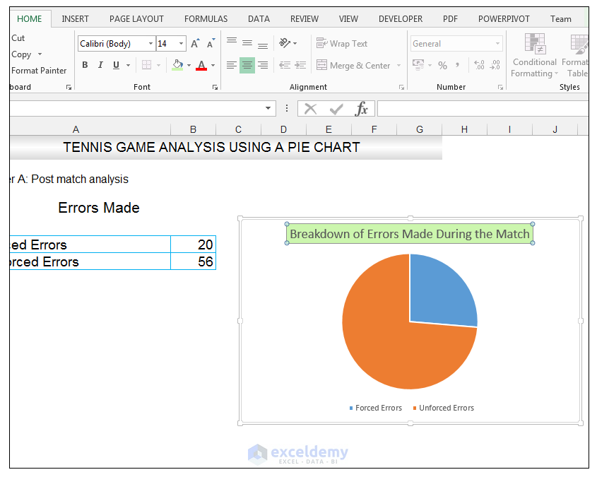
How to Make a Pie Chart in Excel & Add Rich Data Labels to ...
How to Overlay Charts in Microsoft Excel - How-To Geek In the Change Chart Type window, select Combo on the left and Custom Combination on the right. Create your chart: If you don't have a chart set up yet, select your data and go to the Insert tab. In the Charts section of the ribbon, click the drop-down arrow for Insert Combo Chart and select "Create Custom Combo Chart."
Adjusting the Angle of Axis Labels (Microsoft Excel)
Tree Maps Data Labels and Tables Formatting/Sorting Errors after ... Tree Maps Data Labels and Tables Formatting/Sorting Errors after Windows 11. My Tree Map in Excel and Powerpoint after the Windows 11 update does not order my tables from smallest/largest value correctly, nor allow me to right-align my data labels, nor does it spell out the data label name.
Label line chart series
Excel Charts with Shapes for Infographics - My Online Training Hub How to Build Excel Charts with Shapes Start by inserting a regular column chart. Then insert the shape you want to use. Make sure it's roughly the same size as the largest column in your chart. CTRL+C to copy the Shape > Select the columns in the chart > CTRL+V to paste the shape. Tip: add data labels and remove the gridlines and vertical axis.

Adding rich data labels to charts in Excel 2013 | Microsoft ...

Google Workspace Updates: Get more control over chart data ...

Custom Excel Chart Label Positions • My Online Training Hub
Align data labels in a graph so they are all along the same ...
How to move chart X axis below negative values/zero/bottom in ...
How to I rotate data labels on a column chart so that they ...

Custom data labels in a chart
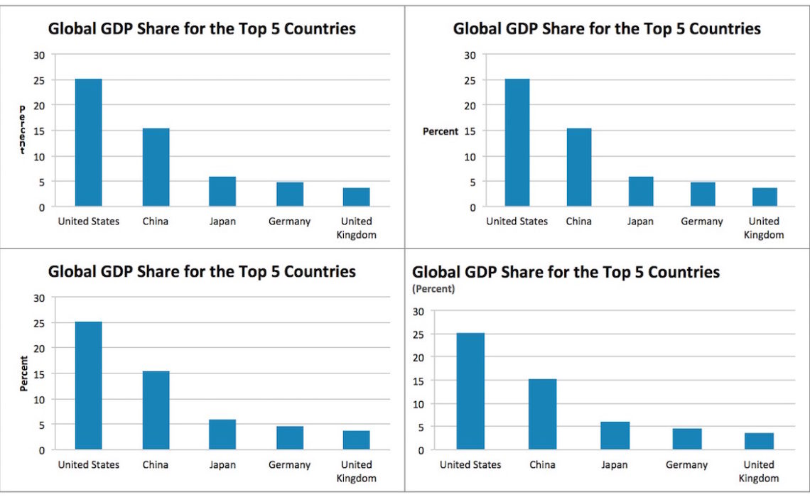
Where to Position the Y-Axis Label - PolicyViz

quick tip: left uppermost align title text — storytelling ...

Change the format of data labels in a chart

Align Chart Titles, Labels, and Legends with Arrow Keys in Excel
How to move Y axis to left/right/middle in Excel chart?
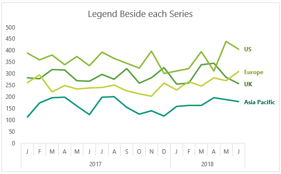
Dynamically Label Excel Chart Series Lines • My Online ...
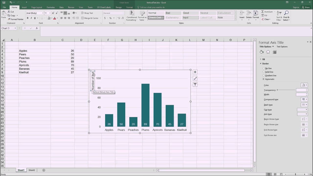
Adding horizontally-aligned y-axis titles to charts in Excel 2016

Excel 2019 - hw does one left-justify the text in an Excel ...

Bar charts with long category labels; Issue #428 November 27 ...

Adding rich data labels to charts in Excel 2013 | Microsoft ...

Google Workspace Updates: Get more control over chart data ...
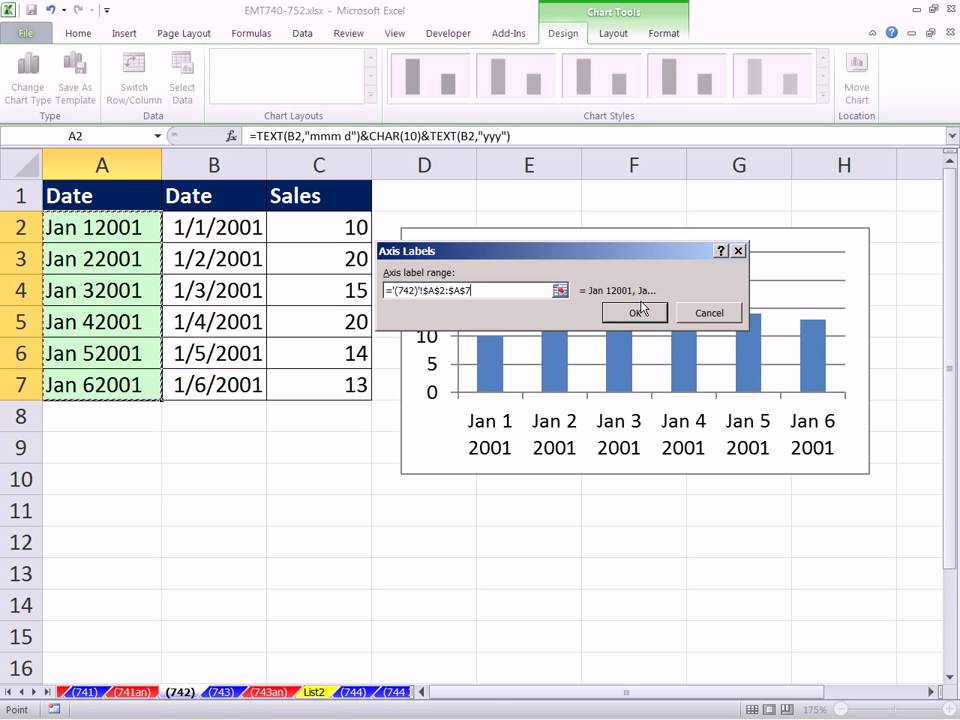
Excel Magic Trick 742: Wrap Text In Chart Label Using CHAR function and Code 10
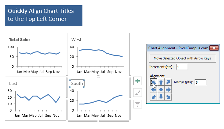
Move and Align Chart Titles, Labels, Legends with the Arrow ...

How to add or move data labels in Excel chart?

How to Add Total Data Labels to the Excel Stacked Bar Chart ...
Excel Chart Secondary Axis • My Online Training Hub
text within a data label in pie chart in excel 2010 doesn't ...

How to Customize Your Excel Pivot Chart Data Labels - dummies
Post a Comment for "44 align data labels in excel chart"